Universal Invariant Networks Through a Nice Commutative Diagram
\(\newcommand{\RR}{\mathbb{R}}\) \(\newcommand{\NN}{\mathbb{N}}\)
\(\newcommand{\mc}{\mathcal}\)
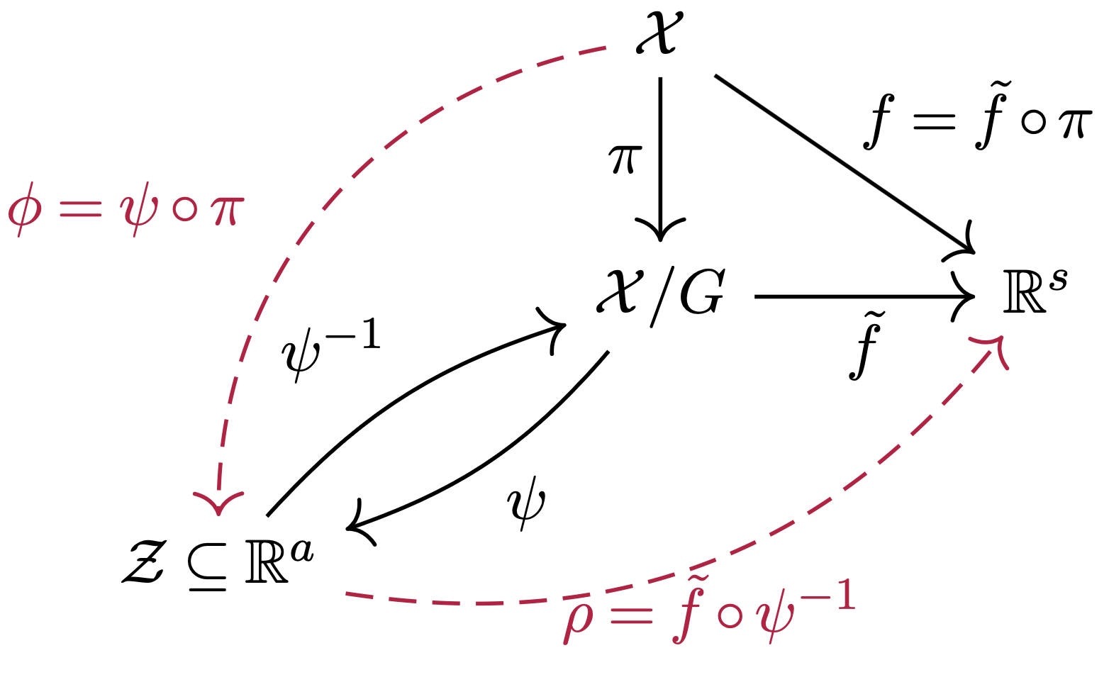
When working on a project with group invariant neural networks, I found myself repeatedly using essentially the same steps to prove many different results on universality of invariant networks. I eventually realized that these steps could be captured in the following commutative diagram:
What’s more: this commutative diagram helps simplify and unify previous proofs of results in the study of invariant neural networks. Plus, it gives a blueprint for developing novel invariant neural network architectures.
In this post, I will explain what this all means. This should be of interest to people who like invariant neural networks, or are curious about applications of some basic topology, algebra, and geometry to the study of neural networks.
Definitions
First, an invariant neural network is a neural network \(f\) such that certain transformations of its inputs do not affect its outputs. We denote the set of transformations as \(G\), and assume that \(G\) is what is known as a group in algebra. Then a neural network \(f\) that is \(G\)-invariant satisfies \(f(gx) = f(x)\) for any \(g \in G\).
For instance, if \(f\) is an image classifier, then certain translations of the input images should not change the output of \(f\); a picture \(x\) with a duck in the bottom right corner and a picture \(gx\) with the same duck in the top left corner should both be classified as having a duck. Thus, \(f\) should approximately be invariant to the group \(G\) of translations. Convolutional neural networks for image classification are approximately invariant to translations.
We say that a network is universal if it can compute all continuous functions that we care about. In particular, we say that a \(G\)-invariant network architecture is universal if it can express any continuous \(G\)-invariant function.
In the commutative diagram above, \(\mathcal X\) is the domain that our input data lies on. We will assume \(\mc X \subseteq \RR^D\) is embedded in some Euclidean space of dimension \(D\). The quotient space \(\mathcal X / G\) is the set of all equivalence classes of inputs under the transformations of \(G\). In other words, it is the space \(\mathcal X\), but where \(gx\) is viewed as equal to \(x\) for any \(g \in G\). The quotient map \(\pi: \mathcal{X} \to \mathcal{X}/G\) is the map that sends an \(x \in \mathcal{X}\) to the equivalence class of all inputs that it can be transformed to, \(\pi(x) = \{ gx : g \in G\}\). Thus, \(\pi\) is \(G\)-invariant.
Mathematical notes
We will generally assume \(G\) is a finite or compact matrix Lie group. A lot can be said when \(\mathcal X\) is just a topological space, though we will assume \(\mc X\) is embedded in some Euclidean space so that we can process our data with standard neural networks. A more detailed discussion of assumptions can be found in the appendix of our paper [Lim et al. 22], but the topological assumptions are generally very mild.
Commutative Diagram
A commutative diagram is a diagram where you can take any path through arrows and arrive at the same result. Let \(f: \mathcal{X} \to \mathbb{R}^s\) be any \(G\)-invariant continuous function. As an example, the above commutative diagram says that there is an \(\tilde f\) such that \(f = \tilde f \circ \pi\), and also an invertible \(\psi\) such that \(\tilde f \circ \psi^{-1} \circ \psi \circ \pi = f\).
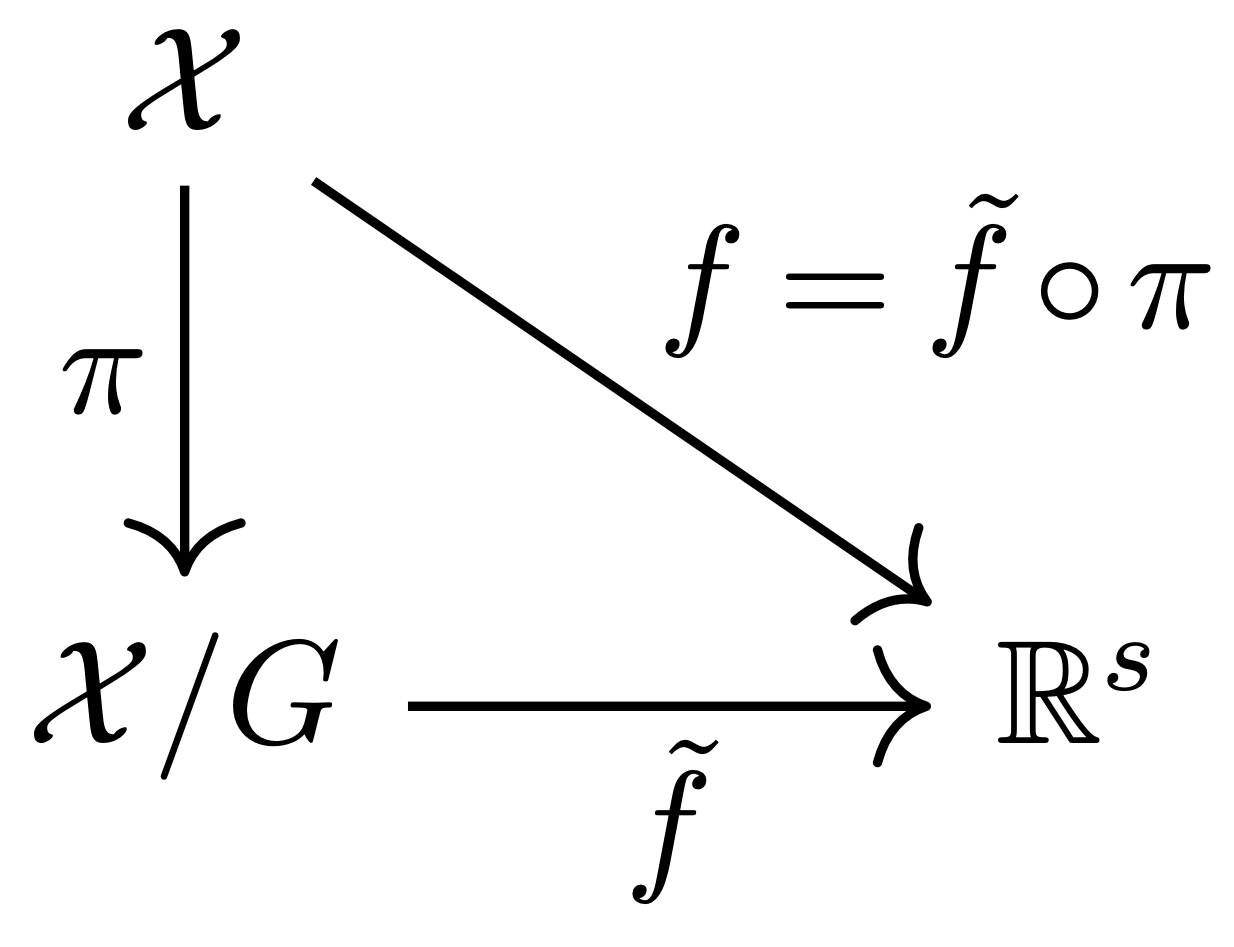
First, consider the subdiagram shown here. This captures the so-called universal property of quotient spaces; for any continuous \(G\)-invariant function \(f: \mc X \to \RR^s\), there exists a unique continuous function \(\tilde f: \mc X / G \to \RR^s\) on the quotient space such that \(f = \tilde f \circ \pi\). However, this does directly not help us to parameterize \(G\)-invariant functions \(f\), as the quotient space \(\mc X / G\) that the \(\tilde f\) are defined on may look rather non-Euclidean (recall that the quotient space consists of equivalence classes of data points), so we may not know how to parameterize functions on such a domain.
Thus, we will want a topological embedding \(\psi : \mc X / G \to \mc Z \subseteq \RR^a\) of the quotient space into some Euclidean space \(\RR^a\), which means \(\psi\) is a continuous bijection with continuous inverse \(\psi^{-1}\). This brings us closer to parameterizing \(G\)-invariant neural networks. The two functions denoted with dashed red arrows in the commutative diagram are parameterized by neural networks: \[ \begin{align*} \phi & = \psi \circ \pi : \mc X \subseteq \RR^D \to \mc Z \subseteq \RR^a \\ \rho & = \tilde f \circ \psi^{-1}: \mc Z \subseteq \RR^a \to \RR^s. \end{align*} \] Of course, \(f = \tilde f \circ \pi = \tilde f \circ \psi^{-1} \circ \psi \circ \pi = \rho \circ \phi\). Note that \(\rho\) and \(\phi\) are compositions of continuous functions, so they are both continuous. Also, their domains are Euclidean spaces, so we can approximate them with standard neural network operations. \(\rho\) can be parameterized by an unconstrained neural network. However, \(\phi\) is required to be \(G\)-invariant, so it seems that we have not made progress, as our original goal was to parameterize \(G\)-invariant functions by neural networks. The next section shows how we can utilize structure in \(\phi = \psi \circ \pi\) to parameterize \(G\)-invariant neural nets.
Finding a quotient space embedding with structure
To parameterize the \(G\)-invariant \(\phi = \psi \circ \pi\), we need to find some structure in \(\psi \circ \pi\) that handles the \(G\)-invariance. For instance, for processing sets we want permutation invariance, and we can show that in this case for input \(x \in \RR^n\) (which represents a set of \(n\) real numbers) we may write \(\phi(x) = \sum_{i=1}^n \varphi(x_{i})\) for some suitable \(\varphi\) that does not have the \(G\)-invariance constraint. Thus, we may then parameterize \(\varphi\) with a standard neural network. There are different ways to find such structure in \(\phi\) or the quotient space embedding.
One way to find structure in \(\phi\) is to find structure in a generating set of \(G\)-invariant polynomials. A generating set \(p_{1}, \ldots, p_{l}\) of the \(G\)-invariant polynomials is a set of \(G\)-invariant polynomials such that every other \(G\)-invariant polynomial \(p\) can be written as a polynomial in \(p_{1}, \ldots, p_{l}\). Lemma 11.13 of [González and de Salas 03] shows that the map \(h: \mc X \to \RR^l\) given by \(h(x) = (p_{1}(x), \ldots, p_{l}(x))\) induces a topological embedding \(\tilde h: \mc X / G \to h(\mc X)\) such that \(h = \tilde h \circ \pi\). Thus, choosing \(\psi = \tilde h\) as our topological embedding above, we have that \(\phi(x) = h(x)\), so \(\phi\) contains all the structure that \(h\) does. This is why for the permutation invariant case, we can choose \(\phi(x) = \sum_{i=1}^n \varphi(x_{i})\); as the polynomials of the form \(p_{k}(x) = \sum_{i=1}^n x_{i}^k\) for \(k=1, \ldots, n\) are generating polynomials of the permutation invariant polynomials, we can write \[\phi(x) = h(x) = (p_{1}(x), \ldots, p_{n}(x)) = \sum_{i=1}^n (x_{i}, \ldots, x_{i}^n),\] so letting \(\varphi(x_{i}) = (x_{i}, \ldots, x_{i}^n)\), we have a nice sum decomposition structure on \(\phi\).
While this use of the \(G\)-invariant polynomials is theoretically general, it can be difficult to use in practice besides for particular choices of \(G\). This is because generators of \(G\)-invariant polynomials can be difficult to find for different \(G\), and they can take complicated forms with high degree polynomials (of up to degree \(|G|\) by Noether’s bound 1). Thankfully, efficiently-computable generators are well known for two of the cases we consider below: when the groups are for permutation symmetries or for rotation/reflection symmetries.
Parameterizing with neural networks
Suppose that the data domain \(\mc X\) is compact, and that we have some structure such that \(\phi\) can be universally approximated by neural networks. Then \(\rho\) and \(\phi\) can be universally approximated by a neural network.
This is due to an application of standard universal approximation results, which say that neural networks can universally approximate continuous functions with domains that are compact subsets of some Euclidean space. If \(\mc X\) is compact, then one can show that \(\mc X / G\) is compact and thus \(\mc Z\) is compact. Hence, \(\phi: \mc X \to \mc Z\) and \(\rho: \mc Z \to \RR^s\) are continuous functions on compact subsets of Euclidean spaces, so they are amenable to approximation by neural networks.
Application 1: Deep Sets
We now give more details on the application of this commutative diagram to neural networks on sets. If we represent a set of \(n\) elements as a vector \(x \in \mathbb{R}^n\), then we want any function on the set to not depend on the order of the elements. Thus, letting \(G = \mathbb{S}_n\) be the group of permutations on \(n\) elements, we want a function \(f\) on sets to be invariant to permutations \(f(g x) = f(x)\), where \(gx = [x_{g(1)}, \ldots, x_{g(n)}]\) permutes the entries of \(x\) by the permutation \(g\).
The invariant DeepSets [Zaheer et al. 17] architecture parameterizes permutation invariant functions as \[ f(x) \approx \rho_\theta\left(\sum_{i=1}^n \phi_\theta(x_{i}) \right),\] where \(\rho_\theta\) and \(\phi_\theta\) are neural networks. Their proof that the architecture is universal uses a few computations and facts about symmetric polynomials (see their Appendix A.2).
We can instead prove universality using the above commutative diagram as follows. We take our generating set of \(G\)-invariant polynomials as the power sum symmetric polynomials: \(p_{k}(x) = \sum_{i=1}^n x_{i}^k\) for \(k=1, \ldots, n\). Thus, we know that in the above commutative diagram, we can write \[\phi = \psi \circ \pi(x) = \begin{bmatrix}\sum_{i=1}^n x_{i} & \ldots & \sum_{i=1}^n x_{i}^n\end{bmatrix} = \sum_{i=1}^n \begin{bmatrix}x_{i} & \ldots & x_{i}^n\end{bmatrix}.\]
Hence, in the DeepSets neural architectures, we can approximate \(\rho_{\theta} \approx \rho\), and \(\phi_\theta(y) \approx \begin{bmatrix} y & \ldots & y^n \end{bmatrix}\), which standard feedforward networks can do, so DeepSets is universal.
We note that this connection to the power sum symmetric polynomials as an embedding of the quotient space is also used in [Finkelshtein et al. 22], see their Appendix C.
Application 2: Rotation and Reflection Invariance
When dealing with certain types of point clouds of points in \(\mathbb{R}^d\), we may want to be invariant to rotations and reflections, which form the group \(G = O(d)\) of orthogonal \(d \times d\) matrices. [Villar et al. 21] proposed to use some classical results in invariant theory to parameterize \(O(d)\)-invariant neural networks. For learning an \(O(d)\) invariant function \(f: \RR^{n \times d} \to \RR^s\) on \(n\) points that satisfies \(f(Q v_{1}, \ldots, Qv_{n}) = f(v_{1}, \ldots, v_{n})\) for any \(Q \in O(d)\), they parameterize \[ f(v_{1}, \ldots, v_{n}) \approx g_{\theta}(V^\top V) = g_{\theta}((v_{i}^\top v_{j})_{i,j=1, \ldots, n}). \] In other words, \(g_\theta\) is a neural network acting on all inner products of two points \(v_{i}\) and \(v_{j}\). [Villar et al. 21] uses an argument based on the Cholesky decomposition to say that allowing \(g_\theta\) to be any arbitrary function gives universality.
To see that we only need continuous \(g_\theta\) and that we can thus use a neural network as \(g_\theta\), we note that the First Fundamental Theorem of \(O(d)\) from invariant theory says that the inner product polynomials \(p_{ij}(v_{1}, \ldots, v_{n}) = v_{i}^\top v_{j}\) are generators of the \(O(d)\)-invariant polynomials. Thus, in the above commutative diagram, we can write \[\phi(x) = \psi \circ \pi(x) = \begin{bmatrix} v_{i}^\top v_{j} \end{bmatrix}_{i,j=1, \ldots, n}.\] So the functions of the form \(\rho(\begin{bmatrix} v_{i}^\top v_{j} \end{bmatrix}_{i,j=1, \ldots, n})\) are universal. As \(\rho\) is unconstrained and continuous, we can approximate it by a neural network \(\rho_\theta \approx \rho\), so the networks of the form \(\rho_\theta( \begin{bmatrix} v_{i}^\top v_{j} \end{bmatrix}_{i,j=1, \ldots, n})\) are universal.
Application 3: Direct Products and Eigenvectors
Our recent paper [Lim et al. 22] inspired this blog post, as I discovered this common pattern underlying the commutative diagram through working on this project. In the paper, we develop universal architectures for a large class of invariances coming from direct products. If \(G_i\) is a group acting on \(\mc X_i\) for \(i=1, \ldots, k\), then the direct product \(G_1 \times \ldots \times G_k\) is the group of tuples \((g_1, \ldots, g_k)\) which acts on \(\mc X_1 \times \ldots \times \mc X_k\) as \((g_1, \ldots, g_k) (x_1, \ldots, x_k) = (g_1 x_1, \ldots, g_k x_k)\). In our Theorem 1 (the decomposition theorem), we show that a continuous function \(f(x_1, \ldots, x_k)\) that is invariant to the large group \(G = G_1 \times \ldots \times G_k\) can be parameterized as \[f(x_1, \ldots, x_k) \approx \rho_\theta\left(\phi_{1,\theta}(x_{1}), \ldots, \phi_{k,\theta}(x_{k}) \right),\] where \(\phi_{i,\theta}\) only needs to be invariant to the constituent smaller group \(G_{i}\), and \(\rho\) is unconstrained. Further, we can take \(\phi_{i,\theta} = \phi_{j,\theta}\) if \(\mc X_{i} = \mc X_{j}\) and \(G_{i} = G_{j}\). We prove this theorem precisely through the same-old commutative diagram, where we show that the \(\phi\) map has a product structure \[\phi(x_{1}, \ldots, x_{k}) = (\phi_{1}(x_{1}), \ldots, \phi_{k}(x_{k})),\] for some \(G_{i}\)-invariant functions \(\phi_{i}\) on the \(\mc X_{i}\).
We proved this result to apply it to a specific invariance arising from learning functions on eigenvectors. For a matrix \(A \in \RR^{n \times n}\) with an eigenvector \(v \in \RR^n\) of eigenvalue \(\lambda\), note that \(-v\) is also an eigenvector of \(A\) with the same eigenvalue. A numerical eigenvector algorithm could have returned either \(v\) or \(-v\), so we want a function \(f\) on eigenvectors \(v_{1}, \ldots, v_{k}\) to be invariant to sign flips: \[f(\pm v_{1}, \ldots, \pm v_{k}) = f(v_{1}, \ldots, v_{k}).\] There are in fact more invariances desired if there is a higher dimensional eigenspace, but we will not cover those here (see [Lim et al. 22] for more on this). This sign invariance is precisely invariance to the action of the group \(G = \{1, -1\}^k = \{1, -1\} \times \ldots \times \{1, -1\}\). Thus, our theorem says that as long as we can parameterize a universal network that is \(\{1, -1\}\) invariant, then we can use that to make a \(\{1, -1\}^k\) invariant function. Invariance to \(\{1, -1\}\) just means that \(h(-x) = h(x)\), so such a function is an even function, which can be simply parameterized as \(h(x) = \varphi(x) + \varphi(-x)\) for some unconstrained \(\varphi\). Thus, we can parameterize sign invariant functions on \(k\) vectors as \[f(v_{1}, \ldots, v_{k}) \approx \rho_\theta\left( \phi_\theta(v_{1}) + \phi_\theta(-v_{1}), \ \ldots, \ \phi_{\theta}(v_{k}) + \phi_{\theta}(-v_{k})\right).\] Note that we can use the same \(\phi_\theta\) for each vector \(v_{i}\) by our decomposition theorem, as \(\mc X_{i} = \mc X_{j}\) and \(G_{i} = G_{j}\) for each \(i\) and \(j\).
Limitations
While I think the strategy based on this commutative diagram may be useful for developing new invariant architectures (especially those that come from direct products of groups), this is far from solving every problem in invariant machine learning. For one, many invariant networks are built from equivariant layers followed by a final invariant pooling. Using equivariance has been shown to significantly improve performance in certain applications (e.g. note the success of networks with convolutional layers that are approximately translation equivariant, or see Figure 7 of [Batzner et al. 22] for an example in molecular dynamics). Also, this is mostly concerned with developing universal architectures, but universality is not sufficient for good performance. Inductive biases can greatly improve the performance of invariant architectures, as can be seen by the success of adding attention modules to Set architectures [Lee et al. 19] [Kim et al. 21] or as we saw by adding message passing to our SignNet architecture for eigenvectors of graph operators [Lim et al. 22]. Even if we do desire universality, this commutative diagram approach may not be computationally useful, as there may be no nice quotient space embedding with structure that we can leverage.
References
[Zaheer et al. 17] Deep Sets.
[Villar et al. 21] Scalars are universal: Equivariant machine learning, structured like classical physics.
[Lim et al. 22] Sign and Basis Invariant Networks for Spectral Graph Representation Learning.
[Finkelshtein et al. 22] A Simple and Universal Rotation Equivariant Point-cloud Network.
[Batzner et al. 21] E(3)-Equivariant Graph Neural Networks for Data-Efficient and Accurate Interatomic Potentials.
[Lee et al. 19] Set Transformer: A Framework for Attention-based Permutation-Invariant Neural Networks.
[González and de Salas 03] C∞-differentiable spaces. Springer.
[Kim et al. 21] Transformers Generalize DeepSets and Can be Extended to Graphs and Hypergraphs.
[Kraft and Procesi 96]. Classical Invariant Theory.
Noether’s bound says that the \(G\)-invariant polynomials of degree at most \(|G|\) generate all \(G\)-invariant polynomials. See e.g. [Kraft and Procesi 96] Theorem 2.↩︎